Paper explained · 20 October 2026
Attention Is All You Need, Explained from the Ground Up
A visual guide to the original Transformer: intuition first, then attention mathematics, tensor shapes, masking, and small PyTorch examples.
Explore this guide
Imagine translating “The animal did not cross the street because it was tired.” Before translating “it,” you need to connect it to “the animal.” Its meaning depends on something several words away.
Now imagine doing that for every part of a sentence: deciding which earlier or later pieces help interpret each token, then using those relationships to write a translation.
That is the problem at the heart of Attention Is All You Need, the 2017 paper by Ashish Vaswani and colleagues that introduced the Transformer. Its central proposal was to build a sequence-to-sequence model around attention, removing recurrence and convolution from the main architecture. Attention existed before this paper; the architecture built around it was the important step. Read the original paper.
This guide starts with an everyday explanation, then works through the actual operations. You do not need to know Transformers already. Familiarity with lists of numbers and basic Python will help; the sections on shapes make the matrix operations explicit.
By the end, you should be able to trace one token through the model, explain the attention equation, distinguish the three attention patterns, and understand what a training step is trying to learn.
1. The problem before the Transformer
A translation system accepts a source sequence and produces a target sequence, often with a different length. For example:
- Source: “I love maths.”
- Target: “J’aime les maths.”
A common approach before Transformers used a recurrent neural network, or RNN. It updated a hidden state one token at a time. To process position 8, it first needed the state from position 7, which needed position 6, and so on.
That creates two difficulties. First, the computations along the sequence depend on one another, limiting parallelism. Second, information about distant tokens has to travel through many recurrent updates. Attention-equipped recurrent models already helped with the second problem by letting a decoder consult source representations directly.
The Transformer took a further step: make attention the mechanism for exchanging information between positions, without a recurrent chain.
This does not mean the model has no layers or dependencies. It means that, within a training layer, representations at many positions can be computed together using matrix operations. The network still processes one layer after another.
2. The whole model before the details
The original Transformer is an encoder–decoder model. Think of the two parts as having different jobs:
- The encoder builds context-aware representations of the source sentence.
- The decoder uses those representations and an existing target prefix to predict the next target token.
“Token” is the right unit here, rather than “word.” A tokenizer can split a word into smaller pieces. For readability, our diagrams use whole words as if they were tokens.
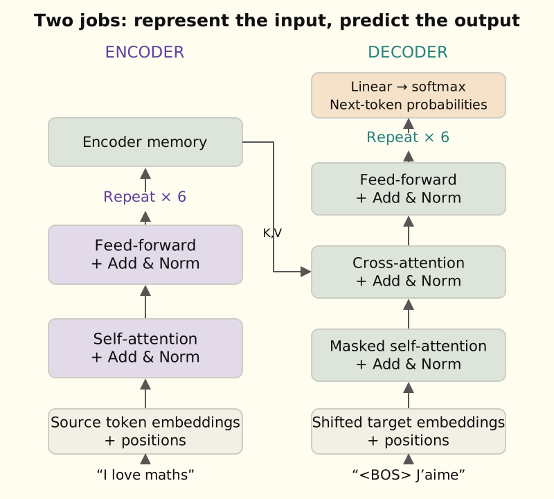
Do not try to memorise every box yet. Follow the information:
- Source tokens become vectors with position information.
- Encoder layers let source positions exchange information.
- The decoder receives the target prefix, also represented as vectors.
- It reads the prefix, consults the encoder, and produces scores over the output vocabulary.
- During generation, one selected token is appended to the prefix and the process repeats.
A useful distinction: the encoder does not generate a finished translation that the decoder tidies up. It provides a sequence of representations that the decoder can repeatedly consult.
3. What a token representation actually is
A model cannot directly calculate with a string such as “animal.” A tokenizer maps text to integer IDs, and an embedding table maps each ID to a learned vector.
If the vocabulary contains $V$ tokens and the representation width is $d_{model}$, the embedding table has shape:
$$E \in \mathbb{R}^{V \times d_{model}}$$Looking up an ID selects a row. At first, those numbers are not useful linguistic descriptions. Training adjusts them, together with the rest of the model, to improve predictions.
For a batch of two sentences with four token positions each, a width of 512 gives a tensor of shape [2, 4, 512]: batch, position, feature.
A feature is not necessarily an interpretable property such as “animal” or “past tense.” Meaning can be distributed across many dimensions. After contextual processing, two occurrences of the same token can have different representations because their surroundings differ.
Why position needs its own signal
If attention only compares token content, it has no built-in notion that one token came first and another came fourth. Reordering the input rows would simply reorder self-attention’s output rows in the absence of position information and position-dependent masking. That property is called permutation equivariance.
The paper adds a positional vector to each token embedding. Its fixed encodings use sine and cosine at different frequencies:
$$PE(pos,2i)=\sin\left(\frac{pos}{10000^{2i/d_{model}}}\right)$$$$PE(pos,2i+1)=\cos\left(\frac{pos}{10000^{2i/d_{model}}}\right)$$Here, $pos$ is the token position, and $i$ selects a pair of feature dimensions. Each pair follows a different rate of change.
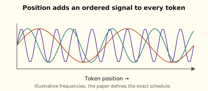
Why add the two vectors? They have the same width, so addition gives each position a representation containing both content and an ordered signal. The network learns to use that combined representation.
The original model scales embeddings by $\sqrt{d_{model}}$ before adding positions. It also applies dropout to the resulting sum. The authors investigated learned positional embeddings too; sine waves are a design choice, not a requirement for every Transformer. Paper, §3.4–3.5.
4. Attention is a learned way to mix information
Here is the simplest useful definition:
For each position, attention calculates how much information to take from each available position, then forms a weighted mixture.
In our opening sentence, the representation of “it” might benefit from information about “animal.” The model does not follow a manually written pronoun rule. Training changes its numerical operations so that useful relationships can emerge.
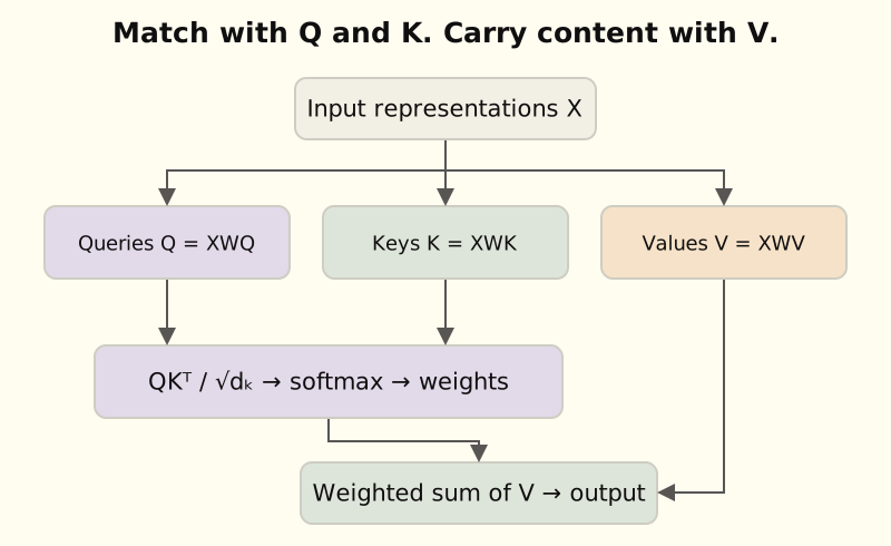
To make the mixing operation flexible, attention uses three roles:
- A query represents what a receiving position is looking for.
- A key represents how a candidate position can be matched.
- A value carries the information contributed if that candidate receives weight.
A library analogy helps: a search request is a query, catalogue information is a key, and the retrieved content is a value. But attention is a soft lookup: it usually mixes several values rather than returning exactly one item.
Where do queries, keys, and values come from?
They are learned projections of representations. In self-attention, the same input matrix $X$ supplies all three:
$$Q=XW^Q,\qquad K=XW^K,\qquad V=XW^V$$The projection matrices are learned parameters. $Q$, $K$, and $V$ are the resulting activations for the current input. There is no external database of fixed keys in ordinary self-attention.
5. The attention equation, one operation at a time
The central equation is:
$$\operatorname{Attention}(Q,K,V)=\operatorname{softmax}\left(\frac{QK^T}{\sqrt{d_k}}\right)V$$Let us unpack it without skipping the dimensions. For one head, suppose there are $T_q$ query positions and $T_k$ key/value positions:
| Quantity | Shape | Meaning |
|---|---|---|
| $Q$ | $T_q \times d_k$ | One query vector per receiving position |
| $K$ | $T_k \times d_k$ | One key vector per candidate position |
| $V$ | $T_k \times d_v$ | One value vector per candidate position |
| $QK^T$ | $T_q \times T_k$ | Every query compared with every key |
| Attention weights | $T_q \times T_k$ | A distribution over keys for each query |
| Output | $T_q \times d_v$ | One mixture of values per query |
The output has one row per query, even when the source and target sequences have different lengths.
Step A: compare each query with each key
The entry at row $i$, column $j$ of $QK^T$ is a dot product:
$$s_{ij}=q_i\cdot k_j$$A larger score gives that key more relative weight for that query after softmax. The learned projections decide what kinds of compatibility produce large scores. It is more precise to call this a learned matching score than a general measure of “word similarity.”
Step B: keep score magnitudes under control
Why divide by $\sqrt{d_k}$? Under the simplifying assumption that query/key components are independent, have zero mean, and unit variance, a sum of $d_k$ products has variance $d_k$. Dividing by $\sqrt{d_k}$ brings that variance back toward 1.
Large score differences can make softmax concentrate almost all its weight on one entry. In saturated regions, its gradients can become very small. Scaling helps control this as head width grows. It does not guarantee a particular distribution or fix every training problem.
Step C: turn each row into weights
For scores $z_1,\ldots,z_n$:
$$\operatorname{softmax}(z)_j=\frac{\exp(z_j)}{\sum_r\exp(z_r)}$$The denominator runs over keys for the same query. Each row sums to 1. Rows are not normalised together, and columns need not sum to 1.
Subtracting the largest score before exponentiation gives the same result and avoids unnecessarily large exponentials. Libraries perform stable versions of this operation.
Step D: mix the values
For query $i$, the result is:
$$o_i=\sum_j a_{ij}v_j$$This is what the final multiplication by $V$ does. Attention weights are not the final representation; they describe how to combine the values into one.
The formula and the three attention roles follow §3.2 of the original paper. The worked example below uses invented vectors.
6. A complete calculation with tiny numbers
Use one query and three key/value pairs:
query = [1, 0]
keys  = [[1, 0], [0, 1], [1, 1]]
values = [[2, 0], [0, 2], [2, 2]]
The query–key dot products are $[1,0,1]$. Since $d_k=2$, divide them by $\sqrt{2}$ to obtain approximately $[0.707,0,0.707]$.
Softmax gives approximately $[0.401,0.198,0.401]$. The result is therefore:
$$0.401[2,0]+0.198[0,2]+0.401[2,2]\approx[1.604,1.198]$$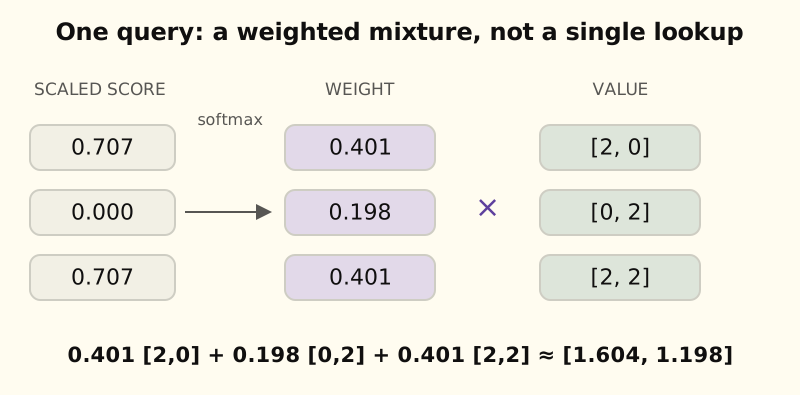
Try changing the attention scores
These are invented two-dimensional vectors, chosen to make the calculation visible. Adjust a score and watch the mixture change.
| Key | Value | Weight |
|---|---|---|
| 1 | [2, 0] | |
| 2 | [0, 2] | |
| 3 | [2, 2] |
Output ≈ [1.604, 1.198]. Weights sum to 1.
Try making all three scores equal. You will get equal weights and the ordinary average of the values. Then increase one score. The result moves toward its value. Finally, block the third key: its weight becomes exactly zero and the other weights are renormalised.
The same operation in PyTorch
import math
import torch

q = torch.tensor([[1., 0.]])
k = torch.tensor([[1., 0.], [0., 1.], [1., 1.]])
v = torch.tensor([[2., 0.], [0., 2.], [2., 2.]])

scores = q @ k.T / math.sqrt(q.shape[-1])
weights = scores.softmax(dim=-1)
output = weights @ v

print(weights)  # approximately [[0.4011, 0.1978, 0.4011]]
print(output)   # approximately [[1.6044, 1.1978]]
These vectors are manually chosen. In a trained model, their values depend on embeddings, earlier layers, and learned projections. The arithmetic stays the same.
7. Why use multiple attention heads?
A single attention operation produces one pattern of mixing per query. Multi-head attention creates several learned projections and computes several such patterns in parallel.
The paper’s base model uses representation width 512 and eight heads, with query/key/value width 64 per head. Eight outputs of width 64 are concatenated into width 512, then transformed by an output projection. Paper, §3.2.2.
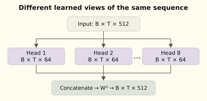
With a batch, the common shape progression is:
Projected Q:     [B, Tq, 512]
Split heads:     [B, 8, Tq, 64]
Attention map:   [B, 8, Tq, Tk]
Head outputs:   [B, 8, Tq, 64]
Join heads:     [B, Tq, 512]
Output project: [B, Tq, 512]
Heads can learn different relationships. That does not mean head 1 is guaranteed to learn grammar and head 2 is guaranteed to resolve pronouns. Their functions emerge during training, may overlap, and need not have simple human-readable labels.
The output projection matters: it allows information from different head outputs to be combined. Concatenation alone only places them beside each other.
8. Three attention patterns, not three different formulas
The original model uses the same attention mechanism with different sources and visibility rules:
| Pattern | Queries come from | Keys and values come from | Allowed information |
|---|---|---|---|
| Encoder self-attention | Source representations | The same source sequence | All non-padding source positions |
| Decoder self-attention | Target-prefix representations | The same target sequence | Current and earlier non-padding positions |
| Encoder–decoder cross-attention | Decoder representations | Final encoder representations | All non-padding source positions |
In cross-attention, a decoder query asks: given the target prefix so far, what source information is useful now? The key/value sequence can have a different length from the query sequence.
The encoder can read a complete source sentence because it is already available. A decoder predicting the next target token cannot read that answer from a later target position. That leads to masking.
9. Masking: prevent information leakage before softmax
During training, complete target sentences are available. If the decoder could attend to future target positions, it could use information that will not exist when generating a translation.
A causal mask blocks those future connections. In a score matrix, rows are receiving query positions and columns are key positions they might read.
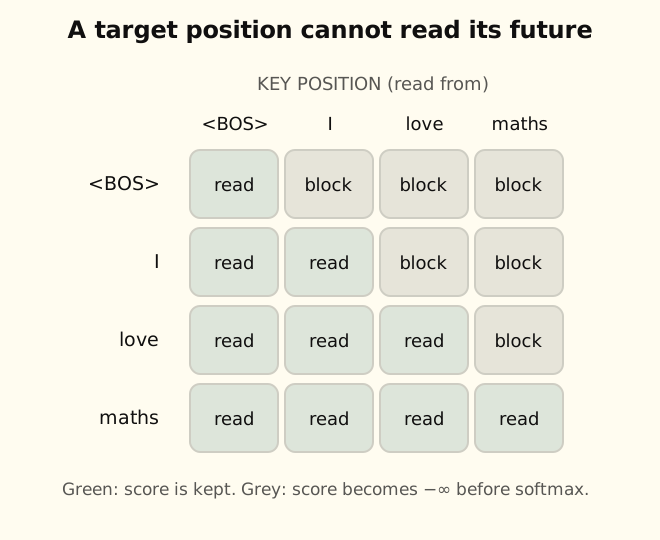
Blocked scores become $-\infty$ before softmax. Since $\exp(-\infty)=0$, those positions receive zero probability, while the remaining positions still sum to 1.
length = 4
allowed = torch.ones(length, length, dtype=torch.bool).tril()
scores = torch.randn(length, length)
weights = scores.masked_fill(~allowed, float('-inf')).softmax(-1)

assert torch.all(weights.triu(diagonal=1) == 0)
assert torch.allclose(weights.sum(-1), torch.ones(length))
Setting a blocked score to zero would not work: softmax would assign it nonzero weight. Zeroing weights after softmax would also lose normalisation unless you renormalised them.
Padding is a different mask
Sentences in a batch often have different lengths. Padding makes a rectangular tensor, but padding tokens must not be treated as meaningful evidence. A key-padding mask prevents attention from reading those positions.
For batched heads, a source mask might have shape [B, 1, 1, S], broadcasting over heads and query positions. A target mask combines [1, 1, T, T] causal visibility with [B, 1, 1, T] target-key visibility.
Every query needs at least one available key. A row of entirely $-\infty$ scores has no valid softmax distribution. The downloadable example rejects that situation explicitly. Outputs at padded target-query positions are ignored in the loss.
Mask conventions differ between APIs. In this article’s custom code, True means allowed. PyTorch’s functional scaled-dot-product attention also uses that Boolean convention, whereas Boolean masks for nn.MultiheadAttention use True to block. Check the specific API rather than copying a mask blindly. PyTorch attention documentation.
10. Attention is only part of a Transformer block
Attention exchanges information between positions. The rest of the block transforms that information and helps the network train.
The position-wise feed-forward network
After attention, every position passes through the same two-layer network:
$$\operatorname{FFN}(x)=\operatorname{ReLU}(xW_1+b_1)W_2+b_2$$The base model expands width 512 to 2048, applies ReLU, then returns to width 512. Parameters are shared across positions within a layer, but not across all layers.
from torch import nn

ffn = nn.Sequential(
    nn.Linear(512, 2048),
    nn.ReLU(),
    nn.Linear(2048, 512),
)
This network does not mix positions on its own: it transforms the features at each position separately. Attention is the part that moves information between positions.
Residual connections
A residual connection adds a sublayer’s result to its input, preserving a direct path for information and gradients:
$$x+\operatorname{Sublayer}(x)$$For this addition to work, both terms must have the same representation width.
Layer normalisation and dropout
The original paper uses post-norm:
$$\operatorname{LayerNorm}\left(x+\operatorname{Dropout}(\operatorname{Sublayer}(x))\right)$$Layer normalisation operates across a token’s feature dimension, using that token’s feature mean and variance, followed by learned scale and shift. It is not normalisation across all tokens or the whole batch.
Dropout randomly removes some contributions during training as regularisation. It is disabled during evaluation. The paper applies residual dropout and dropout to the embedding-plus-position sums. Paper, §3.1, §3.3 and §5.4.
Many later architectures use pre-norm, different activations, or different position encodings. Those can be useful changes, but they are not the exact block described in this paper.
11. What happens during training?
The model is trained on source–target pairs. The encoder sees the source, while the decoder receives the target shifted right.
If the desired target is “I love maths,” the decoder input and labels are:
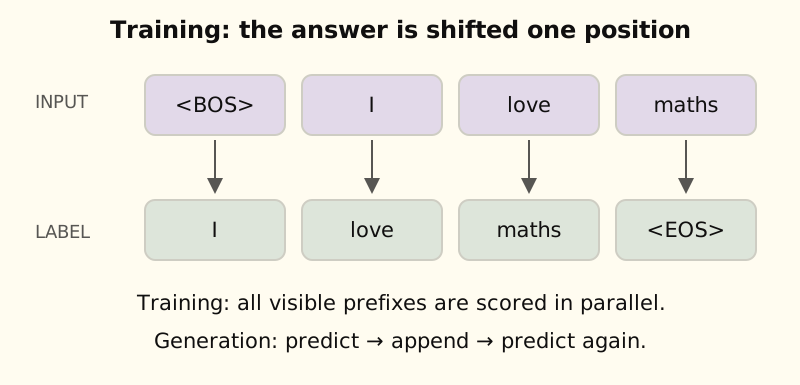
At the input position containing “love,” the label is “maths.” The model knows the prefix ending in “love,” so that prediction is valid. Allowing it to read the following “maths” input would reveal its answer.
The decoder produces a vector of vocabulary scores, or logits, at every position. Cross-entropy penalises assigning low probability to the correct next token. Padding labels are excluded.
In notation, the sequence probability factorises as:
$$p(y\mid x)=\prod_{t=1}^{T}p(y_t\mid y_{A small training step
The downloadable Python example defines a readable encoder–decoder Transformer. It includes learned Q/K/V projections, multi-head attention, sinusoidal positions, post-norm blocks, and both causal and padding masks.
Here is how to use it for a single illustrative step. The IDs are invented, not a real translation dataset:
# TinyTransformer is defined in the downloadable example.
# PAD=0, BOS=1, EOS=2; other IDs are ordinary toy tokens.
model = TinyTransformer()
source = torch.tensor([[3, 4, 2, 0], [5, 6, 7, 2]])
target = torch.tensor([[1, 8, 9, 2, 0], [1, 10, 11, 12, 2]])

decoder_input = target[:, :-1]
labels = target[:, 1:]
logits = model(source, decoder_input)  # [2, 4, 16]

loss = torch.nn.functional.cross_entropy(
    logits.reshape(-1, logits.size(-1)),
    labels.reshape(-1),
    ignore_index=0,
)
optimizer = torch.optim.Adam(model.parameters(), lr=1e-3)
optimizer.zero_grad()
loss.backward()
optimizer.step()
Pass raw logits to PyTorch cross-entropy; do not apply softmax first. Gradients then flow through the output layer, decoder, cross-attention, encoder, and embeddings, adjusting parameters toward better predictions. Cross-entropy API.
The tiny model uses width 32 and two layers so the computation is approachable on CPU. One step on arbitrary IDs does not produce a translator. It demonstrates the complete information flow and training objective. For readability, it omits attention-weight dropout and does not reproduce the paper’s full optimisation recipe.
12. Why generation is still sequential
Training can score many target positions together because the correct target prefix at each position is supplied, and masking enforces the information boundary.
During generation, the next token does not exist yet:
- Encode the source.
- Start the target prefix with a beginning token.
- Run the decoder and inspect the final position’s vocabulary scores.
- Select a token and append it.
- Repeat until an end token or length limit is reached.
Greedy selection chooses the highest-scoring token. Beam search keeps several candidate prefixes; the original paper used beam search for translation. Sampling is another strategy, common in later generative applications.
Thus, parallel training across known positions does not mean parallel generation of an unknown autoregressive output. Caching decoder keys and values can avoid repeating some work, but each new output token still depends on the earlier generated prefix.
13. The training recipe and what the paper showed
Architecture alone is not the whole experiment. The paper also specifies Adam settings, an increasing-then-decreasing learning-rate schedule, dropout, and label smoothing. Paper, §5.
The learning rate grows linearly during warmup and then decays in proportion to the inverse square root of the step count:
$$\operatorname{lr}=d_{model}^{-1/2}\min\left(\operatorname{step}^{-1/2},\operatorname{step}\cdot\operatorname{warmup}^{-3/2}\right)$$The paper uses 4,000 warmup steps, Adam with β₁ = 0.9, β₂ = 0.98, and ε = 10⁻⁹, and a base-model dropout rate of 0.1. Warmup makes the initial learning rate small, then increases it. The later decay reduces update size over time. Label smoothing, with ε = 0.1 in the paper, assigns some target probability mass away from the correct class, reducing pressure to become completely confident in one label.
The original experiments focused on machine translation. The reported Transformer-big result reached 28.4 BLEU on WMT 2014 English–German, trained on eight P100 GPUs over about 3.5 days. Those are the paper’s historical experimental results, not a score produced by this tutorial or a measure of general language understanding. BLEU compares generated translations with references through n-gram overlap and a length penalty. Paper, §6.1.
14. What made this design useful—and what it costs
Self-attention gives distant positions a direct connection within a layer. It also replaces a time-step recurrence with matrix operations that can be parallelised effectively during training.
But the full attention map has $n^2$ entries for a length-$n$ sequence. For $B$ batches and $H$ heads, the straightforward implementation materialises a [B, H, n, n] tensor. Doubling the sequence length quadruples the number of pairwise scores.
The attention-mixing computation costs approximately $O(n^2d)$; projections and feed-forward layers add other costs, including terms proportional to $nd^2$. “The Transformer is faster” therefore needs context: sequence length, representation width, hardware, implementation, and whether you mean training or generation all matter.
Attention weights are also not a complete explanation of a model’s decision. Values, output projections, residual paths, later layers, and the training objective all affect the eventual prediction. A bright cell in an attention map shows a strong routing weight in that head, not proof of a causal or human-like explanation.
15. The original Transformer and the models that followed
It is easy to read the paper through today’s chatbots and accidentally mix architectures.
| Model family | Typical attention structure | Typical role |
|---|---|---|
| Original encoder–decoder Transformer | Bidirectional source encoder, causal target decoder, cross-attention | Sequence-to-sequence tasks such as translation |
| Encoder-only models | Bidirectional self-attention | Producing contextual representations; task depends on training objective |
| Decoder-only models such as GPT | Causal self-attention, typically without a separate source encoder | Predicting the next token from a prefix |
The paper’s central mechanism remains recognisable across these families, but their information access and training objectives differ. GPT is not simply the complete original model renamed.
Likewise, the title is not a claim that literally every useful computation is attention. The architecture still contains embeddings, position signals, feed-forward networks, residual connections, normalisation, and output layers.
16. Check your understanding
Try answering before expanding each explanation.
Why does attention normalise over keys rather than query positions?
Each query needs its own distribution over the information sources it may read. Normalising across queries would instead make different receiving positions compete for a given key.
If Q, K, and V all come from X, why have three projections?
A position's matching request, its matching description, and the content it contributes serve different roles. Separate learned projections let those roles differ while remaining trainable together.
Why is the causal mask allowed to include its diagonal?
The token at the current decoder input position is already known. Because labels are shifted, the model is predicting the following token. The future input position containing that answer must be blocked.
Could the decoder use self-attention alone to translate?
A decoder can model target-language patterns from its prefix, but it needs access to the source to condition a translation on that particular input. In this architecture, cross-attention supplies that connection.
If a head gives a token 90% weight, does that prove the token caused the final answer?
It shows a strong routing weight in that head, but the value vectors, output projection, residual connections, other heads, and later layers also affect the answer. An attention weight alone does not establish a causal explanation of the complete prediction.
Why can we train many target positions together but generate only one new position at a time?
Training has the reference target sequence, so all shifted prefixes can be evaluated together under a causal mask. Generation must first produce a token before that token can become part of the next prefix.
A mental model to keep
A token begins as an embedding plus position information. Attention lets it collect a learned mixture of information from allowed positions. Feed-forward layers transform that mixture; residual paths and normalisation support the repeated computation. The encoder builds source context, and the decoder uses it with a target prefix to predict what comes next.
If you can explain what a position is allowed to read, how its weights are calculated, and what those weights mix, you have the central mechanism. The rest of the paper gives that mechanism a trainable architecture and tests it on a concrete task.
Sources and further exploration
- Vaswani et al., Attention Is All You Need (2017). The primary source for the architecture, equations, training recipe, and reported translation results.
- Paper in HTML. Read §3 after the architecture sections above, §4 for the computational comparisons, and §5–6 for the experiments.
- PyTorch scaled-dot-product attention and MultiheadAttention. Pay particular attention to mask conventions.
- Download the educational PyTorch implementation. Includes the numerical example and a small encoder–decoder forward/backward step.
- My language-model implementation project. A related exploration of GPT-style components and task adaptation.
All diagrams on this page are original explanatory illustrations. The tiny vectors, simplified sentences, and interactive controls are teaching examples, not attention maps measured from a trained language model.