Introduction
Tensile testing is one of the most fundamental tests in materials science and mechanical engineering. It measures how a material responds to being pulled apart until it breaks. This analysis transforms raw machine data—force and displacement—into meaningful mechanical properties that engineers use for design and quality control.
This guide explains the scientific methodology behind the Tensile Test Analysis Dashboard, covering everything from basic stress-strain calculations to advanced techniques like sliding window regression for E-Modulus determination.
1. Fundamental Concepts: Stress and Strain
Before calculating advanced properties, we must convert raw “Machine Data” (Force and Displacement) into “Material Properties” (Stress and Strain).
A. Engineering Stress ($\sigma$)
Stress represents the internal resistance of a material to an applied force. Unlike “Force,” Stress is independent of the sample’s size, allowing us to compare a thin film to a thick block.
Formula: $$\sigma = \frac{F}{A_0}$$
Where:
- $F$: Force applied by the machine (converted from mN to Newtons)
- $A_0$: Original Cross-Sectional Area ($Width \times Thickness$)
- Unit: MegaPascals (MPa), equivalent to $N/mm^2$
B. Engineering Strain ($\epsilon$)
Strain measures how much the material has stretched relative to its original length ($L_0$).
Formula: $$\epsilon = \frac{\Delta L}{L_0} \times 100$$
Where:
- $\Delta L$: Change in length (Displacement measured by the machine)
- $L_0$: Initial Gauge Length (default is 10.0 mm)
- Unit: Percentage (%) or absolute (decimal)
2. Pre-Processing: The “Toe Region” Correction
When a test begins, the curve often starts with a “shallow” or non-linear slope. This is usually caused by the sample “settling” into the machine’s grips or straightening out slack. This phenomenon is called the Toe Region.
Our Calculation: The software uses a Gradient-Based Crop. It calculates the slope at every point and identifies the moment the slope consistently exceeds a threshold (3% of the maximum slope).
- Shift: The software “crops” the data before this point and shifts the entire curve so it starts exactly at (0,0). This ensures our E-Modulus and Yield calculations are not “polluted” by machine slack.
3. Calculating Mechanical Properties
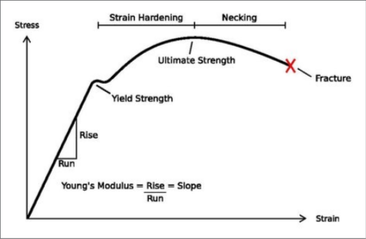
A. Young’s Modulus (E-Modulus)
Young’s Modulus measures the stiffness of the material. It is the slope of the linear (elastic) portion of the curve where the material acts like a spring—returning to its original shape if the load is released.
Our Calculation (Sliding Window Regression): Instead of picking two random points, we use a Sliding Window Search:
- The algorithm scans the first 50% of the curve using a moving window
- It performs a Linear Regression ($y = mx + b$) in every window
- It identifies the window with the highest $R^2$ (Goodness of Fit) and the steepest slope
- Guardrails: If the calculated slope is physically impossible for polymers (e.g., > 15 GPa), it automatically attempts a safer, more localized fit to avoid noise
B. 0.2% Offset Yield Strength ($\sigma_y$)
This is the point where the material stops being “elastic” (spring-like) and starts “plastic” (permanent) deformation. For many materials, this point isn’t a sharp corner, so we use the 0.2% Offset Method.
Our Calculation:
- We take the E-Modulus line and “shift” it to the right by 0.2% strain (0.002 absolute)
- We find where this shifted line intersects the actual Stress-Strain curve
- The Stress value at this intersection is the Yield Strength
C. Ultimate Tensile Strength (UTS)
The maximum stress the material experiences before it begins to fail or “neck” (become thinner in the middle).
Our Calculation: This is simply the Maximum Value of the Stress column after the Toe Region correction.
D. Toughness ($U_T$)
Toughness is the total energy the material can absorb before it actually breaks. A “strong” material might be brittle, but a “tough” material is both strong and ductile.
Our Calculation (Integration): Toughness is the Area Under the Curve from the start of the test until the sample breaks.
- Method: We use the Trapezoidal Rule (calculating the area of tiny vertical slices under the curve and summing them up)
- Unit: $MJ/m^3$ (MegaJoules per cubic meter)
4. Summary Table of Units
| Property | Symbol | Formula | Unit |
|---|---|---|---|
| Stress | $\sigma$ | $Force / Area$ | MPa |
| Strain | $\epsilon$ | $\Delta L / L_0$ | % |
| E-Modulus | $E$ | $\Delta \sigma / \Delta \epsilon$ | GPa |
| Yield Strength | $\sigma_y$ | 0.2% Offset Intercept | MPa |
| Toughness | $U_T$ | $\int \sigma , d\epsilon$ | $MJ/m^3$ |
Key Takeaways
- Tensile testing transforms raw force-displacement data into comparable material properties
- The Toe Region correction ensures accuracy by removing machine artifacts
- Modern algorithms like sliding window regression provide more reliable E-Modulus calculations
- Understanding these properties is essential for material selection and engineering design
This analysis methodology is implemented in Python for the Tensile Test Analysis Dashboard, combining classical engineering principles with modern data science techniques.